Incredible Out-of-the-Box Time Series Analysis with Python and TabPFN: Say Goodbye to Tedious Setups and Hyperparameter Wrangling

Data scientists and analysts are frequently asked for accurate forecasts to help management make better business decisions. But many time series analysis models and tools tend to bog them down with complex setups and long waits at every stage.

What if they have a model that's easy to run and provides accurate forecasts out-of-the-box without fine-tuning, hyperparameter tuning, or complex setup? What if they could generate reliable baseline results quickly on modest datasets, freeing you up for more in-depth analyses?

This is the promise of TabPFN, a new foundational model that could boost your productivity by enabling rapid time series analysis. In this article, we take a deep look into TabPFN for time series forecasting tasks using Python. We explain why we like it, why you should adopt it in your business, how it beats other models and AI assistants, how to use and fine-tune it, and how it works under the hood.

What is Time Series Analysis?

Time series analysis consists of systematically understanding some phenomenon's behaviors and patterns over time.

In the example analysis below, long-term trends, periodic repetitions, correlations over different durations, and future forecasts are conspicuous and can probably be estimated by most people by simply eyeballing the data.

However, most real-world data is rarely this obvious. The data is often very messy and noisy, and most real-world phenomena involve a lot of correlated factors and complex nonlinear relationships. Time series analysis helps us systematically tease out temporal patterns from such messy data.

Where is Time Series Forecasting Used?

Time series forecasting is invaluable to every business. Some common industry uses are outlined below.

• Retail: In retail, forecasting is used to predict:
  
  • Foot traffic and sales by product category, SKU, store, region, and other granularity levels is very common
  • Demand and inventory levels to optimize warehousing costs without stockouts
  • Sales outcomes due to product promotions and discounts
• Ecommerce: Ecommerce use cases are similar retail but some unique forecasting goals include:
  
  • Website visitors broken down by origin like organic search, ads, or social media
  • Conversions
  • Customer lifetime value and churn
  • Ad spend returns
• Health care: The health care ecosystem involves forecasting related to public health policies, medical treatments, drugs, and insurance, such as:
  
  • Spread of infectious diseases
  • Medical outcomes like changes in vital signs, deterioration, or readmission
  • Hospital resource demands like beds, drugs, and equipment
  • Length of hospital stay for insurance forecasts
• Finance: Finance is one of the primary users and innovators of forecasting techniques. They predict:
  
  • Macroeconomic indicators like inflation, GDP, and unemployment rates
  • Asset prices of stocks, bonds, currencies, and more
  • Volatility and fluctuations for robust risk management
  • Interest rates and bond yields
  • Credit risks due to borrowers defaulting

Let's see how TabPFN helps you implement forecasting for these and other real-world use cases.

What is TabPFN?

TabPFN — for tabular prior-data fitted network (PFN) — is a transformer-based foundation model that can accurately predict tabular values (regression) and classify tabular data.

TabPFN-TS uses the same model out of the box for time series forecasting without any pre-training on time series data, either real-world or synthetic. TabPFN's unique training methodology on tabular data turns out to be so effective that it excels even at time series forecasting. You just need to reframe it as a tabular regression problem and do a little feature engineering.

In the rest of this article, we refer to this family of models as TabPFN and analyze its capabilities as well as usage in depth.

How Good is TabPFN? Why Should You Use TabPFN?

Let's look at all the benefits of TabPFN for time series analysis.

Versatile Universal Forecasting Model

TabPFN is not just an ordinary forecasting model but a foundational model capable of universal forecasting, analogous to foundational large language models (LLMs) like GPT-4 or Gemini. It has comprehensive knowledge of all the typical structures, patterns, dynamics, and transitions that are seen in any time series data from any industry or phenomenon.

It builds up this knowledge by training on about 130 million datasets synthetically created by a powerful data generation algorithm.

We explain this data generation algorithm and comprehensive knowledge later in Under the Hood.

Addresses Common Pain Points of Data Scientists and Analysts

TabPFN addresses many common pain points of data scientists and analysts to improve their productivity and reduce frustrations.

• Data wrangling: Messy data like missing or irregular timestamps and different timestamps for different columns are common problems. TabPFN is inherently robust against such messy data. Additionally, TabPFN itself can be used for imputing missing or irregular values.
• Feature engineering: Most forecasting models require addition of a large number of lagged features, rolling window features, and more. TabPFN doesn't need any of them except for a few calendar-based features which can be added easily using its helper functions.
• Inconsistent programming interfaces: A major problem is that different libraries and model types — statistical, machine learning (ML), or deep neural networks — require different programming interfaces and data formats. Ensembling often involves custom glue code. TabPFN ameliorates all this by following the familiar fit-predict semantics of scikit-learn and providing built-in ensembling interfaces. Since it's a general-purpose tabular regression model, it inherently supports exogenous input variables for univariate forecasting.
• Costly model training and hyperparameter tuning: A major time waster with many ML models is the need to first train them on your dataset's structure and columns. Tuning gradient boosting machines and deep learning models involves time-consuming searches for optimum parameters like learning rates, layer sizes, dropout, sequence lengths, tree depth, and more. However, TabPFN does in-context learning during inference itself. It can learn any arbitrary table structure and relationships without any traditional training or hyperparameter tuning at all.
• Built-in ensemble for inference: To improve inference accuracy, TabPFN features a built-in post-hoc ensemble. By default, this involves creating an ensemble of 4 TabPFN models for classification tasks and 8 for regression tasks (this number is controlled by the n_estimators parameter). TabPFN then runs a forward pass through each of these models and averages their results. The input data is slightly modified for each model in the ensemble, effectively achieving data augmentation during in-context learning. Additionally, a dedicated post-hoc ensemble estimator is available, which allows for ensembling more models, potentially with more varied hyperparameters, and offers greater control over scoring and other ensembling strategies.

Using the online TabPFN inference service, your data scientists and analysts can perform quick exploratory forecasts without waiting for a local server to be set up.

Running TabPFN locally for more in-depth secure forecasting is equally simple, thanks to its helper functions. You need not know PyTorch at all — pandas and autogluon knowledge are sufficient.

Top of the GIFT-Eval Leaderboard

TabPFN ranks at the top of the general time series forecasting model evaluation (GIFT-Eval) leaderboard that benchmarks models on datasets from different domains — economy/finance, sales, energy, cloud operations, transport, health care, and nature.

These real-world datasets contain over 144,000 time series and 177 million data points, spanning 10 frequencies, exogenous inputs, and prediction durations from short to long-term forecasts.

TabPFN's high rank is all the more impressive because unlike all the other top models, TabPFN isn't trained on any time series data at all but on general synthetic tabular data!

Let's see TabPFN's rankings in various domains as of April 2025.

HealthCare:

TabPFN is 1st on health datasets like the Project Tycho infectious disease cases and the CDC FluView influenza data.

‍

Economy/Finance:

TabPFN ranks 3rd on banking and finance data like the CIF 2016 datasets.

‍

Nature/Climate/Weather:

TabPFN ranks 3rd on nature and climate forecasting datasets like ERA5 and CMIP6.

High Forecast Accuracy

The paper compares TabPFN accuracy with the following models:

• Statistical time series forecasting models: Seasonal naive, AutoETS, AutoARIMA, and AutoTheta
• Deep neural models: DeepAR (an autoregressive recurrent model) and TFT (a model with recurrent and self-attention layers)
• Pre-trained transformer models: Chronos-Mini and Chronos-Large

They are compared using 24 datasets from the AutoGluon-TS evaluation set.

The metric for point forecast accuracy is the relative mean absolute scaled error (MASE) which scales the absolute forecast errors against those of the seasonal naive baseline. These scores are aggregated over the dataset using geometric mean.

TabPFN shows the lowest forecasting errors. With only 11M parameters, it surpasses Chronos-Mini (20M) by 7.7% and even beats the much larger Chronos-Large (710M) by 3.0%.

The detailed raw MASE scores on the 24 datasets are shown below. You can see that TabPFN scores best on most of them and is closest to the winner in most other cases.

Visualization of TabPFN Forecasts

The paper shows TabPFN forecasts for some difficult time series that showed a high variance in their MASE scores, indicating that there were significant differences between models. Below are the TabPFN forecasts for data where its score was closest to the 50% percentile (median) score of the MASE distribution for that dataset.

These plots give you an idea of TabPFN's median performance even on difficult data.

Capable of Point and Quantile Forecasts

A powerful feature of TabPFN is its ability to produce both point forecasts and quantile probability forecasts as shown below.

In this diagram:

• 0.1-quantile forecast value means there's a 10% probability that the actual value will be less than or equal to it. Alternatively, there's a 90% chance that actual value will be higher than the 0.1-quantile value. It's the floor of the anticipated range of values.
• Similarly, 0.9-quantile forecast means a 90% chance that the actual value will be less than or equal to it. Alternatively, there's only a 10% chance that actual value will be higher than the 0.9-quantile value. It's the ceiling of the anticipated range of values.
• The 0.5-quantile or median value is the center line of the distribution of forecasted values. There's a 50% chance that actual value will be less than it and a 50% chance that actual value will be more than it. It's treated as the point forecast by TabPFN.

These quantile values allow you to quantify the uncertainty in the forecasting to make more informed, risk-aware decisions.

The spread between these quantiles tells you how uncertain the model is. If the 0.1 and 0.9 quantiles are very close to the point forecast, the model is confident of its forecast. If the 0.1 and 0.9 quantiles are far apart, the model predicts a wider range of possible outcomes, indicating high uncertainty.

Another useful metric is skewness. If the 0.5-to-0.9 gap is larger than the 0.1-to-0.5 gap, the uncertainty is skewed towards higher values. But if the 0.1-to-0.5 gap is larger, the uncertainty is skewed towards lower values.

Benefits of quantile forecasts

Quantile forecasts enable robust risk assessment and risk-aware decision-making as outlined below.

• Risk management: If you need to prepare for a worst-case scenario like low sales or low resource availability, look at the lower quantiles like 0.1 or 0.2.
• Opportunity planning: If you want to plan for high demand, look at the higher quantiles like 0.8 or 0.9.
• Inventory management: The quantile forecasts enable intelligent business decisions. You may decide to stock enough inventory to meet demand up to the 0.7-quantile forecast, which means you expect to meet demand 70% of the time and are ok with stockouts 30% of the time. But if stockouts are very costly, you may want to stock enough inventory up to the 0.9-quantile forecast.
• Resource allocation: You may plan server capacity up to the 0.8- or 0.9-quantile forecast to minimize the chances of overload.

Built-In Support for Univariate Forecasting With Exogenous Variables

TabPFN is inherently capable of univariate forecasting with exogenous variables. An important thing to remember about TabPFN is that it's a model for any kind of tabular regression. Univariate forecasting with exogenous variables is just a subset of tabular regression where some of the variables are of a temporal nature and influence the output in addition to its own past values. So you don't need separate covariate regressors like some other models do. This makes TabPFN extremely powerful compared to traditional forecasting machine learning (ML) models.

For example, a timestamp is simply transformed into a couple of calendar-based features/columns. Any other relevant domain-specific variables that influence the dependent variable just become additional features/columns. TabPFN doesn't care about the task or nature of the data — it just sees everything as a table.

You may be wondering how TabPFN can handle the arbitrary number of columns you supply at inference time even though it never saw them at training time. Traditional ML models like random forests can't do that — they need to know the table structure beforehand during training.

TabPFN can do it because of the power of the transformer architecture and in-context learning (ICL). As an analogy, consider how an LLM handles a prompt during inference. It dynamically determines attention weights between the tokens of that prompt and pushes new attention-weighted representations of the tokens through the other layers. 

Similarly, given a data table during inference, TabPFN's special self-attention layers for tabular data dynamically determine:

1) How each cell in a row of that particular table attends to every other cell in the same row

2) How each cell in a column of that particular table attends to every other cell in the same column

ICL enables the input time series data to have arbitrary columns up to a maximum of 500 features and about 10,000 rows. The model dynamically learns the intra-row and intra-column relationships for that data directly during inference.

Excellent Zero-Shot Capabilities

Unlike XGBoost and similar models, TabPFN does not need hyperparameter tuning or fine-tuning on every dataset for high accuracy. Its comprehensive pre-training on 130 million synthetic datasets enables excellent zero-shot performance on any out-of-domain time series.

It enables your data scientists to do exploratory data analyses of time series data without wasting time and effort on model setup. There's even a TabPFN online inference service for quick analyses.

In the above graph, TabPFN outscores both Chronos models in zero-shot experiments, proving its strength as a foundation model.

Robustness Against Messy Data

TabPFN is robust against messy data and uninformative features. It automatically imputes missing values in your time series and normalizes features.

Optimized Architecture and Implementation

TabPFN's custom transformer architecture implements performance optimizations like:

• Pre-computed key value matrices for fast self-attention calculations
• Flash attention support
• Optimized layer implementations that use data chunking and in-place tensor modifications to reduce runtime memory consumption

Supports CPU Inference

You can actually run TabPFN forecasting on workstation CPUs without GPUs. Although the time series wrapper tries to prevent this, circumventing it is easy as we shown in tutorial 3 later in this article.

Useful Generative Capabilities

Due to its ability to infer a probability distribution, TabPFN can easily sample that distribution for unsupervised use cases like:

• Missing value imputation for any time series data
• Outlier detection
• Synthetic data generation by TabPFN (note that this is different from the synthetic data generation used to train TabPFN)

No Legal or Licensing Problems

An important business benefit of TabPFN is that since it's not trained on any real-world datasets at all, it's free of legal issues related to datasets that affect other models, such as licensing, privacy, or copyright infringements.

The TabPFN framework, client libraries, and model weights are published under the liberal Apache 2.0 license with just one additional attribution and model naming requirement.

Why TabPFN Beats GPT-4 at Forecasting

General-purpose AI assistants like ChatGPT, GPT-4, or Gemini are simply not trained for handling time series data effectively. They neither understand nor know to look for characteristics like trends and seasonality.

As a simple test, we told ChatGPT to forecast the next five data points based on 200 rows of the UCI household per-minute power consumption data. It not only got the forecast wrong but even the timestamps wrong, though it just had to add 1 minute to the previous timestamp, as shown below.

Gemini 2.5 Pro honestly admitted that it lacked the tools for forecasting and refused. Gemini 2.0 Flash Thinking just timed out. Gemini 2.0 Flash produced some incomplete Python code before reaching its output token limit.

The latest GPT 4.1 model fared better. It got the timestamps and forecast ballparks right. But it used just a small subset of the given data and its reasoning did not inspire confidence, as shown below.

The first five ground truth values are shown below:

Compare the LLM's output to TabPFN's sophisticated point and probabilistic forecasts below based on the exact same data:

We can see that TabPFN's forecast values are closer to the ground truth. 

Since the values stayed fairly flat from 19:00 to 20:43 during the training period (left of the red line), TabPFN's point forecasts also stayed flat (the orange line). But in its probabilistic forecasts (the gray area), it still somehow anticipated the wild fluctuations after 20:50 without encountering it at all in the training data! The probabilistic forecasts ranged between 2.35 - 6.64 while the actual values went as low as 1.6.

Would TabPFN's forecasts improve if we extended the training duration by a day to include those fluctuations? So we asked it to predict the same time next night. That forecast is shown below:

Our assumption that the fluctuations would repeat next night at the same time didn't hold up. However, TabPFN had learned from the additional data and refined its probabilistic range downwards to 1.36 - 5.79.

Benefit of Specialist Forecasting Model like TabPFN over LLM Like GPT-4

Why do even flagship LLMs fail at this? A major reason is that they don't see numbers like we do but merely as collections of text tokens. Look at how they tokenize this simple arithmetic expression:

Each colored group at the bottom indicates a separate token. As Anthropic's recent research on LLM internals showed, even simple addition involves complicated text wrangling inside an LLM's layers to arrive at an answer.

LLMs just don't do basic math well. More complicated math like time series forecasting is simply beyond their capabilities.

In contrast, TabPFN is specially designed for building up comprehensive knowledge about time series concepts like trends and seasonality. Its attention and neural network layers as well as embeddings and internal representations are all laser-focused on time series patterns and contextual information.

Unlike an LLM, it need not waste its internal memory or attention on general knowledge, instruction-following, or human alignment. That's why its 11 million parameters outperform LLMs with hundreds of billions of parameters.

Accuracy

As we saw above, LLMs are very clumsy with math. Plus, an LLM's loss function optimizes it for predicting the most probable next token (basically a categorical distribution), not forecasting the most accurate numerical value.

In contrast, TabPFN is trained on numerical values with the aim of minimizing the errors for real-valued targets.

Explainability of Results

Explainability is critical in domains like finance and retail where you must be able to justify a forecast with solid reasons. Explainability is a key factor behind the popularity of decision-tree-models like XGBoost.

TabPFN has built-in support for explainability and interpretability through integration with techniques like Shapley additive explanations (SHAP). By supporting it, TabPFN provides a reliable neural alternative to other models.

You can get insights on the influence of each feature on each prediction as shown below.

As for LLMs, they do output their reasoning but as we already saw above, their reasoning on forecasting tasks is fundamentally deficient.

Data Confidentiality

A key business benefit of self-hosted open-weight models like TabPFN is that your sensitive business data can remain under your access control policies. This isn't possible with flagship LLMs which are only accessible through their online endpoints.

Who is Already Using TabPFN?

The GIFT-Eval rankings above show us how TabPFN can be used in different domains like health care, finance, sales, energy, transport, and more.

TabPFN for time series data is still very new and only just starting to find traction in the ML and data science community. However, as a tabular inference model, it is already being used in various domains. In this section, we review these uses and identify closely-related forecasting use cases where TabPFN can help.

Insurance

Due to their better predictive power, transformer-based tabular models are being explored for better insurance pricing and predicting claims frequency, severity, and customer demand. TabPFN too can be used for those tasks as well as forecasting:

• aggregate claim counts and aggregate claim costs based on historical trends, seasonality, and macroeconomic factors
• future costs of claims due to inflation in order to determine future premiums
• future policy counts and total written premium

Another research explored various models to identify existing customers who are most likely to purchase a health insurance policy. This can help an insurance company target its cross-selling marketing more effectively. It found that TabPFN achieved the highest prediction accuracy. TabPFN can also be used to forecast demand for health insurance products and churn rate of existing policyholders.

Manufacturing

Equipment faults can lead to expensive repairs and downtime, with equipment maintenance sucking up 15-60% of production costs. Accurate predictive maintenance that detects faults early and enables proactive fixing can cut maintenance costs by 50%.

TabPFN is being used to identify undesirable operating conditions in machinery based on sensor data. TabPFN can also forecast the remaining useful life of components based on historical sensor data.

Health Care

TabPFN is already widely used in health care projects as outlined below.

• Still birth prediction: TabPFN is used for early detection of higher risk of still birth. It can also be used to forecast near-term fetal heart rate patterns to warn of potentially dangerous patterns like prolonged decelerations.
• Predicting cancer patient responses to immunotherapy: TabPFN is used to predict how cancer patients may respond to immunotherapy based on blood test data. TabPFN can also be used to forecast immune profile evolution and clinical outcome trajectory during treatment.

How to Use TabPFN

In this section, we show you the steps for basic forecasting using TabPFN.

You have two choices:

1. Online TabPFN inference service: The easier option is to use the online TabPFN endpoint managed by Prior Labs. Then, you don't need your server or GPU machine to run the model. However, you wouldn't want to upload your confidential data nor any data with personally identifiable information. So you can't use it for any commercial purposes, just for experimental purposes. There are also rate limits. Also, the endpoint doesn't support fine-tuning. It's ideal for data scientists who want to run quick forecasts on experimental data.
2. Self-hosted model: Since TabPFN is an open-source open-weights model, you can forecast on your own servers. All your data remains confidential. This is the right choice if you need TabPFN's capabilities for commercial purposes. The main drawback is the effort needed for model setup and configuration.

Tutorial 1: Forecasting With the TabPFN Inference Service

We'll walk you through using the TabPFN inference service on the same UCI power consumption data above. A demo notebook is already available from the authors but it relies on HuggingFace datasets. Instead, we'll demonstrate using it with your own pandas dataframe.

Step 1: Create an account and get your access token

Sign up with Prior Labs. After signing up, get your access token and store it securely in your environment.

Step 2: Install TabPFN libraries

In your notebook or virtual environment, install the tabpfn-time-series library.

Get the access token from the user or your environment and set it in the library.

Step 3: Load your DataFrame

This depends on where and how your data is stored. See the pandas IO guide.

For this tutorial, we'll get the DataFrame directly from UCI ML's Python library.

In this case, X and y are already pandas DataFrames.

Step 4: Clean the data

Data cleaning is highly domain and problem specific. However, at a minimum:

• Ensure that your data has a "timestamp" column with the pandas datetime type.
• Sort the DataFrame chronologically by the "timestamp" column.
• Replace any messy or invalid target values with NaN.

For this example, we must combine the Date and Time columns into a single timestamp column of type datetime.

Next, add a column named "target" with the values of the target variable ("Global_active_power" in this example). Ensure that any invalid values in the column are replaced by NaN.

Step 5: Create a TimeSeriesDataFrame

We need to create a TimeSeriesDataFrame object from the DataFrame to pass to the model.

First, copy only required rows and columns to a new DataFrame and sort them by timestamp.

Then create the TimeSeriesDataFrame by specifying the data frequency and the list of target values.

Step 6: Create the training and test sets

Use TimeSeriesDataFrame.train_test_split() to create a training set.

Use generate_test_x() to create the test set with all target values cleared.

Step 7: Feature engineering to improve TabPFN's forecasts

TabPFN and its embeddings work better if some calendar features derived from the timestamps are added. They include sines and cosines based on the hour, day of week, day of month, day of year, week of year, and month.

Step 8: Visualize your data

Use the helper functions to visualize your training and test data.

Step 9: Forecasting

Run the TabPFNTimeSeriesPredictor in CLIENT mode to forecast using the online inference service.

‍

The resulting TimeSeriesDataFrame contains point forecasts ("target" column) and quantile forecasts in the columns named 0.1-0.9, as shown below.

Step 10: Visualize the forecasts

Use the plot_pred_and_actual_ts() helper to visualize the point and quantile forecasts as shown below.

Tutorial 2: Forecasting Locally With Self-Hosted TabPFN Model

For local inference, TabPFN currently mandates an Nvidia GPU and CUDA as prerequisites. The code refuses to run on CPUs (see the next tutorial for how to circumvent this).

A modest consumer-grade GPU or Colab's T4 GPU are good enough. The model is only about 44 MB in size.

All the other steps are exactly the same as the previous tutorial using the online service, except for the forecasting step. For running locally, just set the mode to LOCAL instead of CLIENT as shown below.

Tutorial 3: Forecasting With Self-Hosted TabPFN Model on CPU

TabPFN's refusal to run on CPUs is enforced only by the TabPFNTimeSeriesPredictor wrapper and is easily circumvented. The underlying tabular regression logic has no complaints about running on CPUs.

To circumvent it, you don't even need to modify any of the TabPFN libraries. In your client/application code itself, define a custom TabPFNWorker implementation that returns a CPU-compatible regressor.

We must inject this custom worker into the TabPFNTimeSeriesPredictor. For that, first create a predictor with a mock worker.

Then replace the mock worker with your CPU-compatible worker.

You can now use the predictor as usual as shown in the tutorials above. All the forecasting will run on your system's CPUs.

Tutorial 4: TabPFN vs. Chronos

In this tutorial, we try out the Chronos transformer-based models that specialize in time series forecasting in contrast to TabPFN that does tabular data regression.

The newer Chronos-Bolt models like bolt_tiny, bolt_mini, bolt_small, and bolt_base are faster and can run on both CPUs and GPUs. The original Chronos models like chronos_tiny and chronos_mini can run on CPUs while chronos_small, chronos_base, and chronos_large require GPUs.

Chronos can be run using its own framework or via autogluon. We try the autogluon approach here.

First, install the two required packages, autogluon and chronos-forecasting.

After installation, run the same steps of tutorial 1 above till the featurizing step to get train_xtsdf and test_xtsdf.

Then, create a TimeSeriesPredictor and fit your preferred Chronos model on your training data as shown below.

Now, call predict() to generate prediction_length values starting from the end of train_data.

Visualize the predictions.

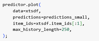
These are the point and quantile predictions of the bolt-small model:

Below are the point and quantile predictions from the larger bolt-base model:

Both Chronos models predicted that the values are more likely to be far above the point forecasts but not far below them. As we saw in tutorial 1, TabPFN better predicted the possibility of values being far below the point forecasts.

A major drawback of Chronos is that univariate regression with exogenous variables involves combining it with additional models to understand the influence of the covariates. In contrast, since TabPFN is a tabular data regressor, it is inherently capable of modeling the influence of exogenous variables on the univariate output variable.

TabPFN Under the Hood

In the following subsections, we provide insights on various internals of TabPFN's architecture and usage.

TabPFN Transformer Architecture

TabPFN uses a custom transformer architecture called the "per-feature transformer." It's an encoder-only architecture by default but can optionally create a decoder too based on a configuration option. In the rest of this article, we'll only explain the encoder-only architecture with settings of available models.

The encoder has 12 "per-feature encoder" layers, each with:

• an inter-feature attention layer with 6 heads for attending between features/columns of a row
• an inter-sample attention layer with 6 heads for attending between records/rows along each column
• a multi-layer perceptron (MLP) layer that calculates the probability distribution using 2 fully-connected hidden layers, each with 768 ReLU neurons
• residual addition for each layer (the input to each layer is added back to its output) 
• a normalization layer after each of the above layers to prevent exploding or vanishing gradients

During inference, the inter-sample attention layer ensures that each test row never attends to any other test rows, only to all the training rows.

Key-Value Caching

During inference, an attention layer can smartly cache the key (K) and value (V) matrices to boost inference speed.

When a new dataset is received for inference, it consists of some in-context training rows and target rows for which values must be forecast. The idea of KV caching is to do a preparation pass where the K and V matrices for all the in-context training rows are computed and cached in memory.

Then for the target rows, it calculates only the query (Q) matrix for each target row and skips K and V computations. Instead, the attention calculation uses the target Q against the cached K and cached V.

Embeddings

Each feature pair or target is transformed into a 192-dimensional embedding by a linear encoder whose weights are learned during the pre-training on synthetic datasets.

Instead of turning each feature into an embedding, TabPFN groups the features into pairs and derives one embedding for each pair of features. The attention is also across these feature groups, not individual features. This grouped encoding apparently improves accuracy compared to deriving one embedding per feature.

Additional feature-level positional embeddings are added to help the model distinguish between different features.

TabPFN Training

TabPFN is a powerful foundational model because it's trained using the prior-data fitted network (PFN) strategy. Let's understand what that means.

The Time Series Generalizability Problem

Time series forecasting is an extremely tough problem to generalize because of the variability in real-world data. The underlying phenomena can be as varied as millisecond-level heart voltages in health care to decades-long macroeconomic metrics in finance. The number of axes of freedoms for time series data is practically infinite in terms of range of values, units, and dynamics.

Compare that to large language models (LLMs) where variability is far less because grammar, semantics, and extant usage greatly restrict the set of probable words that can come next.

What's a good solution for high variability of time series data?

One approach is to train them like LLMs. Gather a huge set of real-world time series data from a large number of domains and pretrain a model on them. However, this brute-force approach has many problems:

• Uncertainty: The entire approach rests on the hope that any new data the model has to predict contains patterns that it has already seen. However, you can never be certain that it has.
• Impracticality: You have to somehow gather millions of real-world datasets to represent most real-world phenomena. It'll involve a lot of effort and cost. You also have to ensure that each dataset has a clean origin and license to avoid legal complications for your model or inference service. In some regulated domains like health care, this may actually be impossible.
• Data leakage: Due to the paucity of real-world datasets, there's a good chance that a dataset already used for training is inadvertently reused during testing, validation, or inference. This can lead to misleading metrics as well as data memorization instead of generalization.

Another popular approach is to train a model for a single narrow problem like heart monitoring, GDP growth, or similar. But that just creates a domain-specific model, not a foundational model.

The PFN Solution for Generalizability

PFN provides an alternative way to create a genuinely generalist foundational model for an entire class of problems like all tabular data tasks or all forecasting tasks. Its training methodology works like this.

1. Focus on abstract patterns and dynamics seen in all time series data

A PFN doesn't try to learn patterns and underlying phenomena specific to any particular domain like health care or finance.

Instead, it treats the set of all datasets of a particular problem type as its "domain." It learns common patterns, structures, and dynamics at that abstraction level to build up a prior distribution in the Bayesian sense.

In TabPFN's case, that abstraction level is the set of all time series data. So it learns about patterns and concepts we associate with abstract time series data, such as:

• General trend: Is the series generally increasing or decreasing?
• Seasonality / periodicity: Do patterns repeat at regular intervals?
• Autocorrelation: How much does the value at one point depend on previous points?
• Noise: How much random fluctuation is there? Is the noise level constant or changing?
• Change points: Are there sudden shifts in the underlying behavior?
• Complexity: How many underlying factors seem to be driving the series?

These are merely illustrative patterns to help you build an intuition about PFNs but aren't necessarily what TabPFN actually learns. Like any typical nonlinear neural network, it will create highly nonlinear combinations of the data and learn their patterns.

This abstract learning is the key to a PFN's generalizability. But where do these 130 million synthetic training datasets come from?

2. Generate synthetic training data

To generate millions of realistic synthetic datasets, TabPFN uses structural causal models (SCM), a framework for representing causal relationships and generative processes. The steps are:

1. For each dataset, sample the characteristic hyperparameters like number of data points, number of features, number of graph nodes, graph topology, or graph complexity.
2. Based on the hyperparameter values, construct a directed acyclic graph of the causal structure.
3. Each node in the graph is a vector representing an abstract cause or effect variable. Each edge is an abstract causal relationship function implemented by: 
   
   • a small neural network with arbitrary linear or nonlinear activations, or
   • a decision tree to encode local rule-based dependencies, or
   • a discretization operation to generate categorical features
4. Each edge also adds some Gaussian noise to introduce randomness into the generated data.
5. Create random noise and propagate it through the graph.
6. The edge functions operate on this random data and generate results.
7. Sample the data from random feature and target nodes.
8. The data representations at these node positions constitutes a sample dataset consisting of feature values and target values generated by the graph's arbitrary functions.
9. Post-process this extracted data to introduce missing values, warping, quantization, and nonlinear distortions. This enables TabPFN to learn how to handle similar issues in real-world datasets.

These steps are repeated millions of times to create a massive corpus of around 130 million synthetic datasets, each with unique causal structure, feature types, and functional characteristics.

Feature Engineering to Increase TabPFN's Predictive Power

TabPFN recommends a set of feature engineering steps to improve forecast quality. The ablation graph above shows how much each feature engineering step improves the accuracy.

For each timestamp, several calendar-based features like the year, the hour of the day, the day of the week, the day of the month, the day in the year, the week of the year, and the month are extracted.

Sine and cosine encoding are applied to each of these features (except the year) to capture their cyclical nature. The period of these derived features is the feature’s natural cycle, such as 7 days for the day of the week.

Additionally, a simple running index feature is added as a temporal reference to track the progression of time across the observations.

How to Fine-Tune TabPFN

In industries like finance, healthcare, retail, and logistics, even a modest improvement in forecasting accuracy can massively boost value or reduce risks. Their forecasting scenarios often involve unique periodic phenomena that a standard model may miss but a fine-tuned model can notice.

Prior Labs, the company behind TabPFN, offers a finetuning program where companies can sign up to create a finetuned model on their proprietary data. 

Benefits of Fine-Tuned TabPFN

Compelling benefits of fine-tuned TabPFN are outlined below:

• Finance: Achieve deeper signal extraction and better risk stratification in credit scoring, fraud detection, default prediction, and more.
• Health care: Improve accuracy for sensitive use cases like clinical outcome modeling, diagnostics, and hospital readmission prediction.
• Retail and e-commerce: Achieve more reliable demand forecasting and pricing optimization.
• Manufacturing and industry: Detect anomalies early and proactively reduce downtime with fine-tuned models for predictive maintenance, quality control, and fault detection.
• Logistics and supply chain: Improve your planning and responsiveness through route optimization, delivery time prediction, and inventory forecasting.

TabPFN Fine-Tuning Workflow

The workflow to fine-tune TabPFN looks like this:

1. Sign up for the fine-tuning service at https://priorlabs.ai/finetuning. Describe your use case and current approaches in the form.
2. The expert team behind TabPFN at Prior Labs sits with your team to evaluate your use case and identify where fine-tuning will drive the most ROI.
3. The Prior Labs team demonstrates what TabPFN can do for your specific challenges.
4. The team signs a non-disclosure agreement with you.
5. The team walks you through the data requirements necessary for the fine-tuning.
6. The data you provide is securely stored in full compliance with the European Union's General Data Protection Regulation (GDPR).
7. The data is ingested by the Prior Labs fine-tuning pipeline.
8. A proprietary, high-performance TabPFN model fine-tuned on your data is created. You have full ownership of your model artifacts.
9. The forecasting results from the fine-tuned model are shared with you. Baseline forecasts and benchmarks against your existing models like XGBoost or LightGBM are also provided.

Additionally, the Prior Labs annual program provides ongoing support and retraining options.

Current Drawbacks of TabPFN

TabPFN is still quite new and undergoing development. You must know some of its current limitations.

Not suitable for long durations

TabPFN currently recommends a maximum of 10,000 rows and 500 features. That translates to about:

• 2.75 hours of per-second data
• 6.9 days of per-minute data
• 416 days of per-hour data

No batch inference support

TabPFN does not currently support batch inference on multiple datasets. Datasets must be supplied one by one.

Higher inference latency

TabPFN's in-context learning approach and the lack of batch inference result in relatively higher latencies compared to some other models.

State-Of-The-Art Time Series Analysis With Python

In this article, we took a deep dive into modern transformer-based approaches for time series forecasting. The versatility of these models, small size, and ability to run on modest hardware boosts the day-to-day productivity of your data scientists and analysts so they can focus on your business goals instead of technical obstacles.

Get in touch with us to help you implement better time series analysis for your business!

References

• Shi Bin Hoo, Samuel Müller, David Salinas, Frank Hutter (2025). "The Tabular Foundation Model TabPFN Outperforms Specialized Time Series Forecasting Models Based on Simple Features." arXiv:2501.02945 [cs.LG]. https://arxiv.org/abs/2501.02945 
• Noah Hollmann, Samuel Müller, Lennart Purucker, Arjun Krishnakumar, Max Körfer, Shi Bin Hoo, Robin Tibor Schirrmeister, Frank Hutter (2025). "Accurate predictions on small data with a tabular foundation model." Nature 637, 319–326 (2025). https://doi.org/10.1038/s41586-024-08328-6
• Samuel Müller, Noah Hollmann, Sebastian Pineda Arango, Josif Grabocka, Frank Hutter (2024). "Transformers Can Do Bayesian Inference."  arXiv:2112.10510v7 [cs.LG]. https://arxiv.org/abs/2112.10510

‍